LX / Tech

Sprache und Technologie - Language and Technology

vectors

noun compounds

Published

May 13, 2026

class: [16830] Sprache und Technologie - Language and Technology:: tutor: frankowsky :: term: SS26 snc: 16175.1

[1] "engine on..."

snc

button.12345
chunk out

index

samling: margin notes general > open

samling

Frankowsky (2022)
- how were dates attested technically?
- what about the decow16 corpus?
  - possible to put that online (term paper) or is it? (Schäfer (2025))
  - corpus formats?

zinsmeister

play

# computing skew divergence score for noun-noun compound vectors
# Q: zinsmeister(2013)


# D(p||q) = Sig^i p^i x log(p^i/q^i)
l1<-c(0.6,0.4,0) # milchzahn
l2<-c(0.25,0.5,0.25) # zahn
l3<-c(0,0,1) # löwenzahn
### test: löwenzahn::ziehen=1 occurence instead 0
l4<-c(0,1,2)
l5<-unlist(lapply(l4,function(x){
x/sum(l4)
}))
########################
# l2 is the reference p
# l1,l3 are the target q probabilities which are projected on /smoothed by reference p
#############################################
lx<-list(list(l2,l1),list(l2,l3),list(l2,l5))
#f<-sum(pi*(log(pi/qi)))
w<-0.9
s1<-lapply(lx,function(l){
  print(l)
#  lapply(l,function(p){
 #   cat("p:",p,"\n")
    s<-array()
    for(i in 1:length(l[[1]])){
      p1<-l[[1]][i]
      q1<-l[[2]][i]
      qi<-(w*q1)+((1-w)*p1) # qi smoothed
      cat("qi:",qi,"\n")
      # s[i]<-sum(pi*log((pi/qi)))
      s[i]<-p1*log(p1/qi)
      cat("s:",s[i],"\n")
    }
    spq<-sum(s)
    cat("skew div:",spq,"\n")
  return(s)
})

[[1]]
[1] 0.25 0.50 0.25

[[2]]
[1] 0.6 0.4 0.0

qi: 0.565 
s: -0.2038412 
qi: 0.41 
s: 0.09922547 
qi: 0.025 
s: 0.5756463 
skew div: 0.4710305 
[[1]]
[1] 0.25 0.50 0.25

[[2]]
[1] 0 0 1

qi: 0.025 
s: 0.5756463 
qi: 0.05 
s: 1.151293 
qi: 0.925 
s: -0.3270832 
skew div: 1.399856 
[[1]]
[1] 0.25 0.50 0.25

[[2]]
[1] 0.0000000 0.3333333 0.6666667

qi: 0.025 
s: 0.5756463 
qi: 0.35 
s: 0.1783375 
qi: 0.625 
s: -0.2290727 
skew div: 0.5249111

names(s1)<-c("milchzahn","löwenzahnA","löwenzahnB")
lapply(s1,sum) #chk.

$milchzahn
[1] 0.4710305

$löwenzahnA
[1] 1.399856

$löwenzahnB
[1] 0.5249111

par(las=2)
boxplot(s1,main="skew divergence scores, reference: zahn")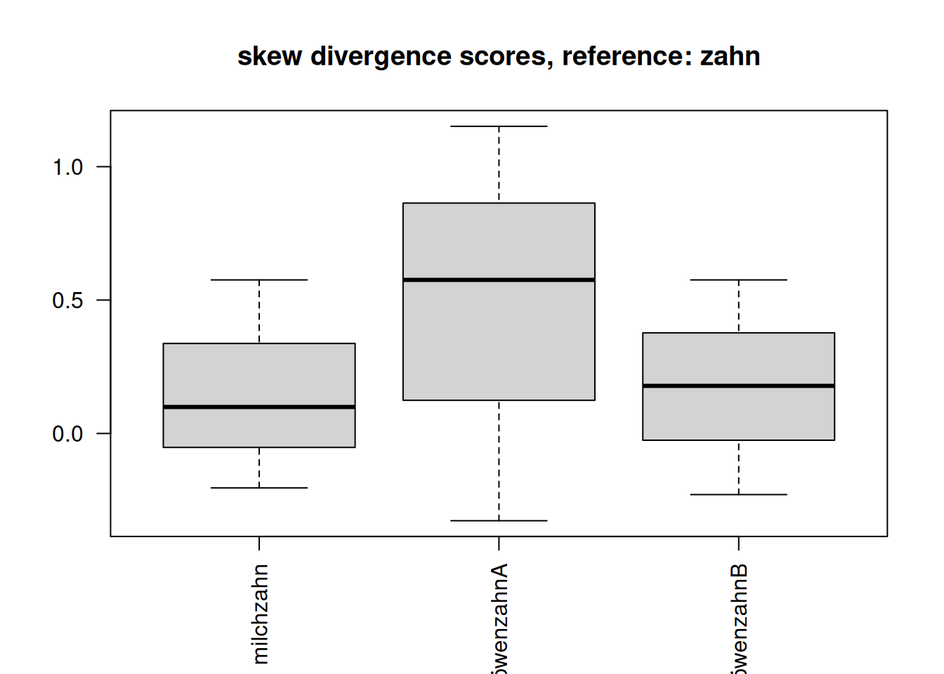

# X = numeric matrix of token embeddings (rows = tokens, cols = features)
# Example:
# X <- as.matrix(df[, -1])
# rownames(X) <- df$t
# l1<-c(0.6,0.4,0) # milchzahn
# l2<-c(0.25,0.5,0.25) # zahn
# l3<-c(0,0,1) # löwenzahn
# ### test: löwenzahn::ziehen=1 occurence instead 0
# l4<-c(0,1,2)
df<-data.frame(token=c("milchzahn","zahn","loewenzahnA","loewenzahnB"),NA,NA,NA)
df[1,2:4]<-l1
df[2,2:4]<-l2
df[3,2:4]<-l3
df[4,2:4]<-l4
#df
X<-as.matrix(df[,-1])
# 1. Row norms (Euclidean length of each token vector)
row_norms <- sqrt(rowSums(X^2))

# 2. Dot-product matrix
#    tcrossprod(X) == X %*% t(X)
dot_products <- tcrossprod(X)

# 3. Outer product of norms
#    Gives all pairwise ||x_i|| * ||x_j||
norm_matrix <- outer(row_norms, row_norms)

# 4. Cosine similarity matrix
cosine_sim <- dot_products / norm_matrix

# 5. Handle rows with zero norm (if any)
cosine_sim[!is.finite(cosine_sim)] <- 0

# 6. Add row/column names
rownames(cosine_sim) <- df$token
colnames(cosine_sim) <- df$token

# Example: similarity between "striker" and "goal"
print(cosine_sim)

            milchzahn      zahn loewenzahnA loewenzahnB
milchzahn   1.0000000 0.7925939   0.0000000   0.2480695
zahn        0.7925939 1.0000000   0.4082483   0.7302967
loewenzahnA 0.0000000 0.4082483   1.0000000   0.8944272
loewenzahnB 0.2480695 0.7302967   0.8944272   1.0000000

cosine_sim["milchzahn", "zahn"]

[1] 0.7925939

# Example: top 5 nearest neighbors for "striker"
nearest_neighbors <- function(token, sim, k = 5) {
  s <- sim[token, ]
  s <- s[names(s) != token]           # remove self-similarity
  s <- sort(s, decreasing = TRUE)
  head(s, k)
}

nearest_neighbors("zahn", cosine_sim)

  milchzahn loewenzahnB loewenzahnA 
  0.7925939   0.7302967   0.4082483

# Normalize counts to probabilities
# P <- counts / rowSums(counts)

# # Cosine similarity
# norms <- sqrt(rowSums(P^2))
# sim <- tcrossprod(P) / outer(norms, norms)
# sim[!is.finite(sim)] <- 0

# Cluster
hc2 <- hclust(as.dist(1 - cosine_sim), method = "average")

# Plot
plot(hc2)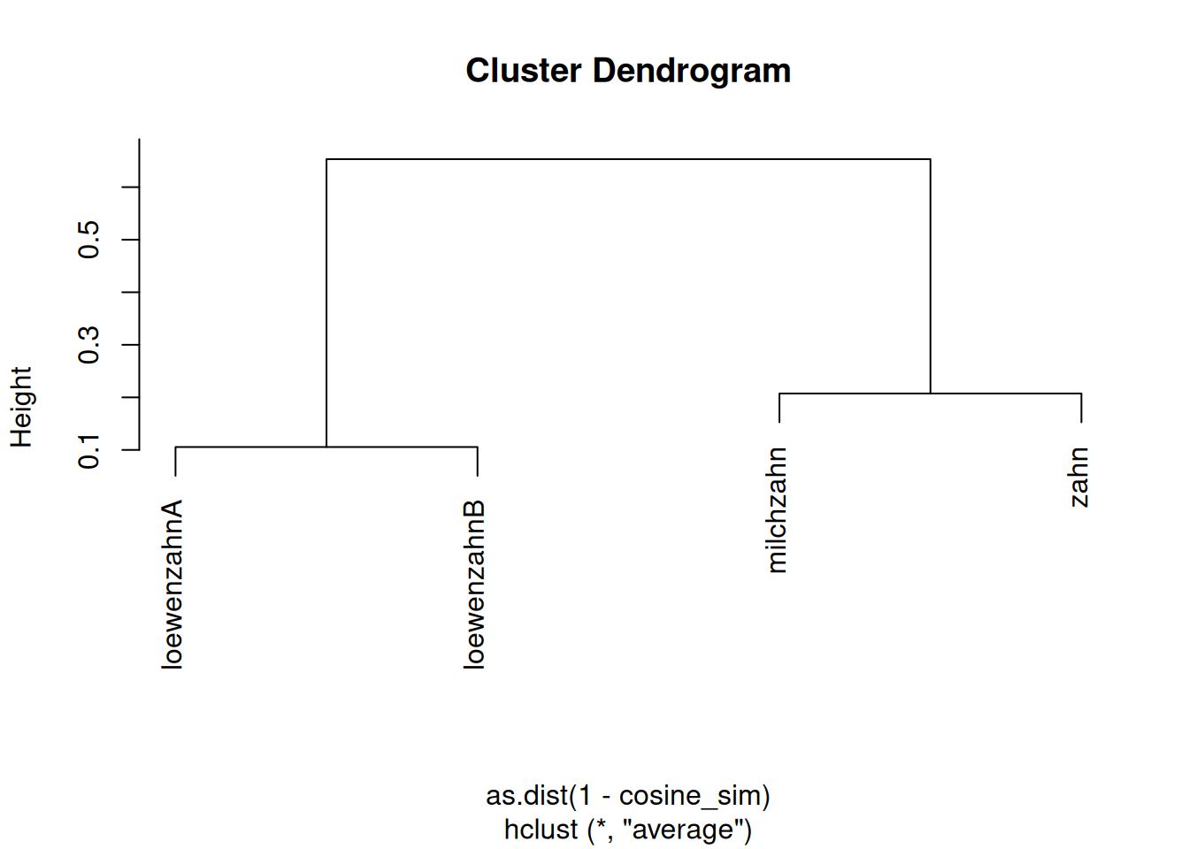

notes

the tokens vector sujet gets interesting if following this theories (LFG: lexical functional grammar) where we may describe token categories in a vector space as well, undisputed of distribution. so if Zinsmeister (2013) investigate on similarity based on distribution of lexical items in a context window (coocurrences) we may also (like in LLM embeddings) make statements about token relatedness based on the vector cosine similarity of tokens semantic / syntactic categories.

the skew divergence approach to measure similiarities of their noun-noun compounds (which nevertheless can be applied to any type of comparison between two probabilty vectors = embeddings) applied by zinsmeister is farely easy to implement in studies since it doesnt afford much manual annotation besides (in their study) to define the contextual words for which a cooccurence is evaluated. playing with the width of a context window, the corpus base or other parameters that constrain cooccurence can yield interesting results in semantic distance of items.

besides, one could also include other parameters next to distributional, including syntactical information, to enlarge the dimension of the vector space and have more finegrained arguments for statements.

References

Frankowsky, Maximilian. 2022. Extravagant Expressions Denoting Quite Normal Entities: Identical Constituent Compounds in German. John Benjamins Publishing Company. https://www.degruyterbrill.com/document/doi/10.1075/slcs.223.07fra/html.

Schäfer, Roland. 2025. What Happened to Webcorpora.org? Roland Schäfer. https://rolandschaefer.net/archives/3663.

Zinsmeister, Heike. 2013. “Corpus–Based Modeling of the Semantic Transparency of Noun–Noun Compounds.” In A Festschrift for Susan Olsen, edited by Holden Härtl. Akademie Verlag. https://doi.org/doi:10.1524/9783050063799.303.